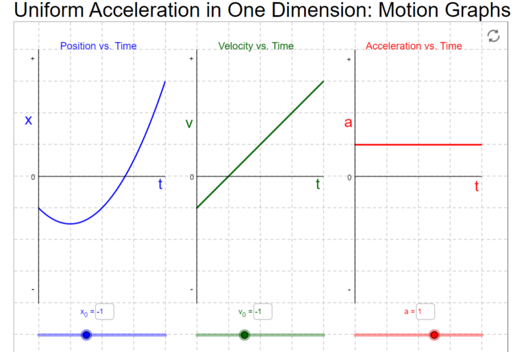
This helps visualize the relationship between x-t, v-t, and a-t graphs for constant-acceleration cases. The acceleration and initial conditions can be independently controlled to show any general type of 1-D motion.

Part of the oPhysics collection.

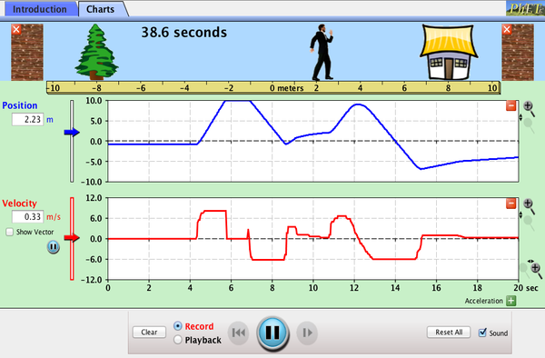
This allows the acceleration of a moving person to be continuously controlled as time elapses. It dynamically illustrates how acceleration, velocity, and position are dependent.

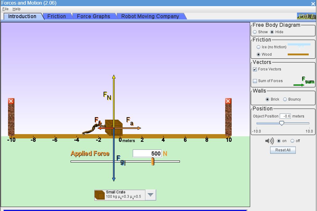
This sim is written in Java. To run on a tablet, click the “Browser-Compatible Version” from the launch screen. It can also be downloaded to a computer to be run offline.

From the PhET collection.

Mohamed – something to figure out (eventually) is that a 2-line header bumps the display text down. Adjust all headers to the same height? Maybe not an issue…

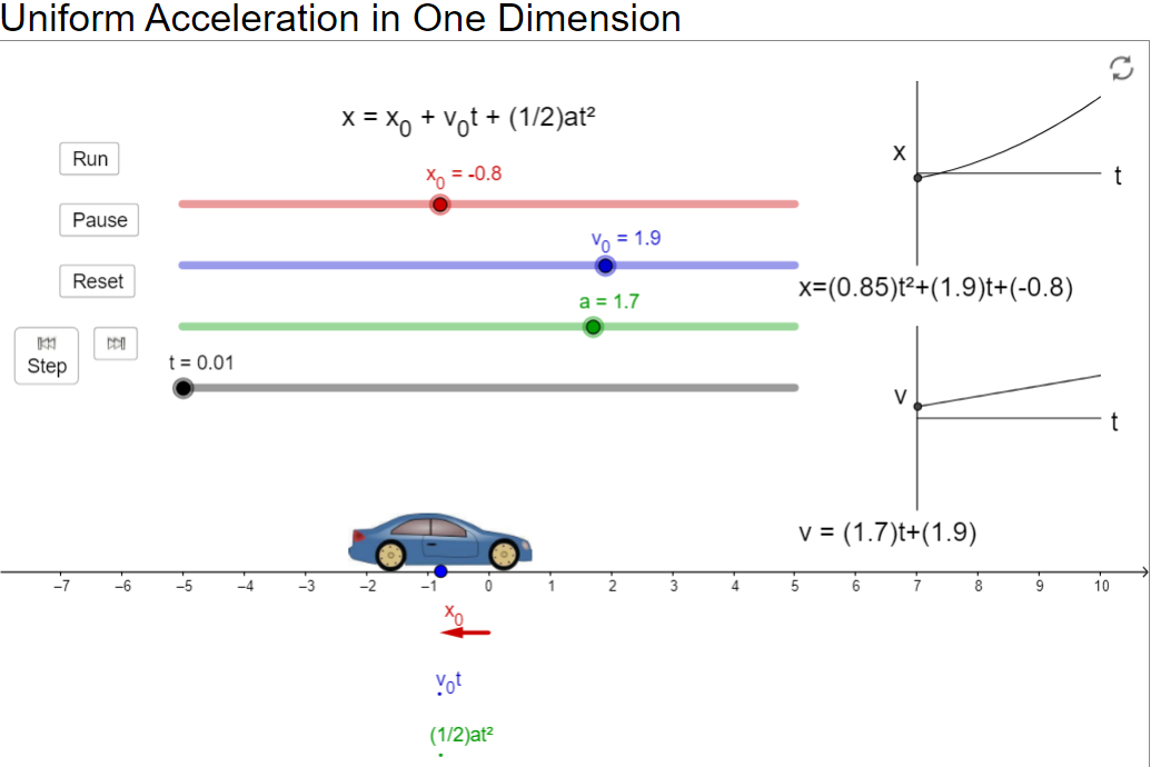
This simulation includes both plots as well as a moving object, given the initial conditions set in the motion. It also includes the relevant algebraic equations of motion for position and velocity.

Part of the oPhysics collection.

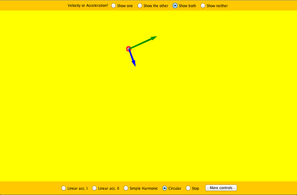
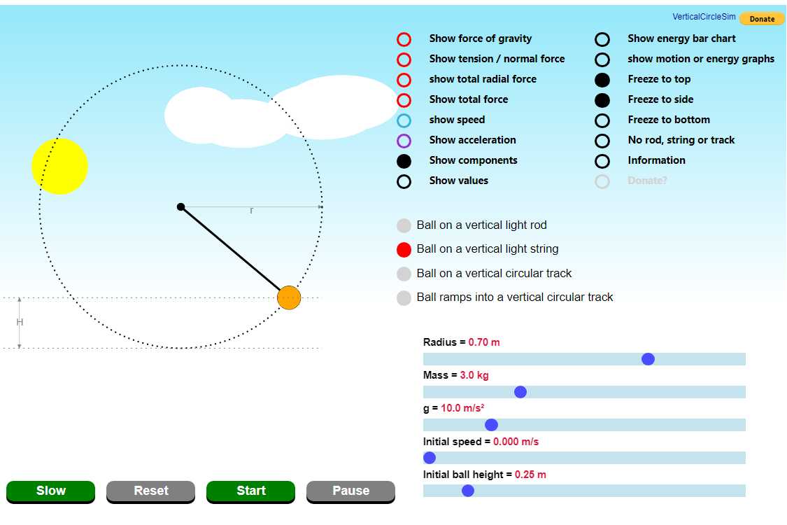
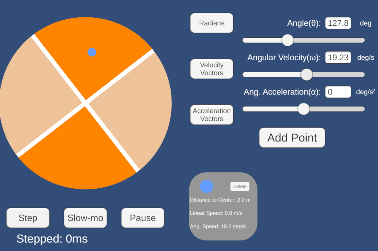
PhET’s Motion in 2D shows the effects of position, velocity, and acceleration on an object in 2D. Motion in 2D has some pre-selected modes of movement which highlight tricky circumstances of movement. The circular movement preset is a great intro to circular motion.

Adapted from PhET.

This simulation shows how projectiles move in 2D. The initial velocity and launch angle can be varied, which affects the projectile’s trajectory.


The resultant x, y, vx, and vy graphs can be shown.


Adapted from PhET.

This simulation shows how projectiles move in 2D. The initial velocity and launch angle can be varied, which affects the projectile’s trajectory.


The resultant x, y, vx, and vy graphs can be shown.


Adapted from PhET.

This simulation shows how projectiles move in 2D. The initial velocity and launch angle can be varied, which affects the projectile’s trajectory.


The resultant x, y, vx, and vy graphs can be shown.


Adapted from PhET.

This simulation shows how projectiles move in 2D. The initial velocity and launch angle can be varied, which affects the projectile’s trajectory.


The resultant x, y, vx, and vy graphs can be shown.


Adapted from PhET.

This simulation shows how projectiles move in 2D. The initial velocity and launch angle can be varied, which affects the projectile’s trajectory.


The resultant x, y, vx, and vy graphs can be shown.


Adapted from PhET.

This simulation shows how projectiles move in 2D. The initial velocity and launch angle can be varied, which affects the projectile’s trajectory.


The resultant x, y, vx, and vy graphs can be shown.


Adapted from PhET.

This simulation shows how projectiles move in 2D. The initial velocity and launch angle can be varied, which affects the projectile’s trajectory.


The resultant x, y, vx, and vy graphs can be shown.


Adapted from PhET.

This simulation shows how projectiles move in 2D. The initial velocity and launch angle can be varied, which affects the projectile’s trajectory.


The resultant x, y, vx, and vy graphs can be shown.


Adapted from PhET.

This simulation shows how projectiles move in 2D. The initial velocity and launch angle can be varied, which affects the projectile’s trajectory.


The resultant x, y, vx, and vy graphs can be shown.


Adapted from PhET.

This simulation shows how projectiles move in 2D. The initial velocity and launch angle can be varied, which affects the projectile’s trajectory.


The resultant x, y, vx, and vy graphs can be shown.


Adapted from PhET.

This simulation shows how projectiles move in 2D. The initial velocity and launch angle can be varied, which affects the projectile’s trajectory.


The resultant x, y, vx, and vy graphs can be shown.


Adapted from PhET.